Applied ML for Cybersecurity | Part 2: Statistical & Bayesian Threat Scoring

I completed the pipeline, structure, and preparation in the first blog, which led me to begin interpretation, risk analysis, and decision-making.
Firstly, I reviewed the dataset constructed in the previous stage. I parsed key log fields including host, process_name, pid, message, and timestamp. From these, I engineered a set of time-based and behavioural features: hour, day_of_week, is_weekend, off_hours, is_system_process, rare_process, first_seen_time, first_seen, session_id, first_seen_session, and count_last_hour.
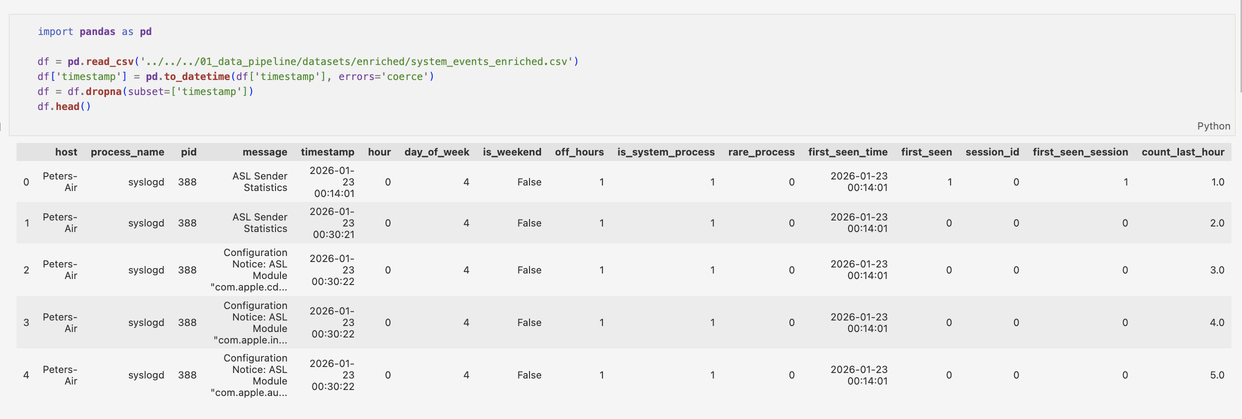
I validated timestamp consistency to ensure temporal consistency as time-based features, such as those previously defined, burst detection and session analysis critically rely on accurate event ordering.
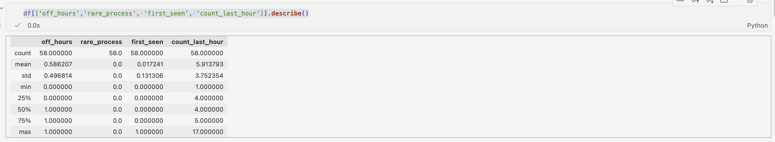
The use of the .describe() function against my data allowed a quick analysis across the statistics:
count→ how many rowsmean→ average valuestd→ standard deviation (spread)min→ smallest value25%→ lower quartile50%→ median75%→ upper quartilemax→ largest value
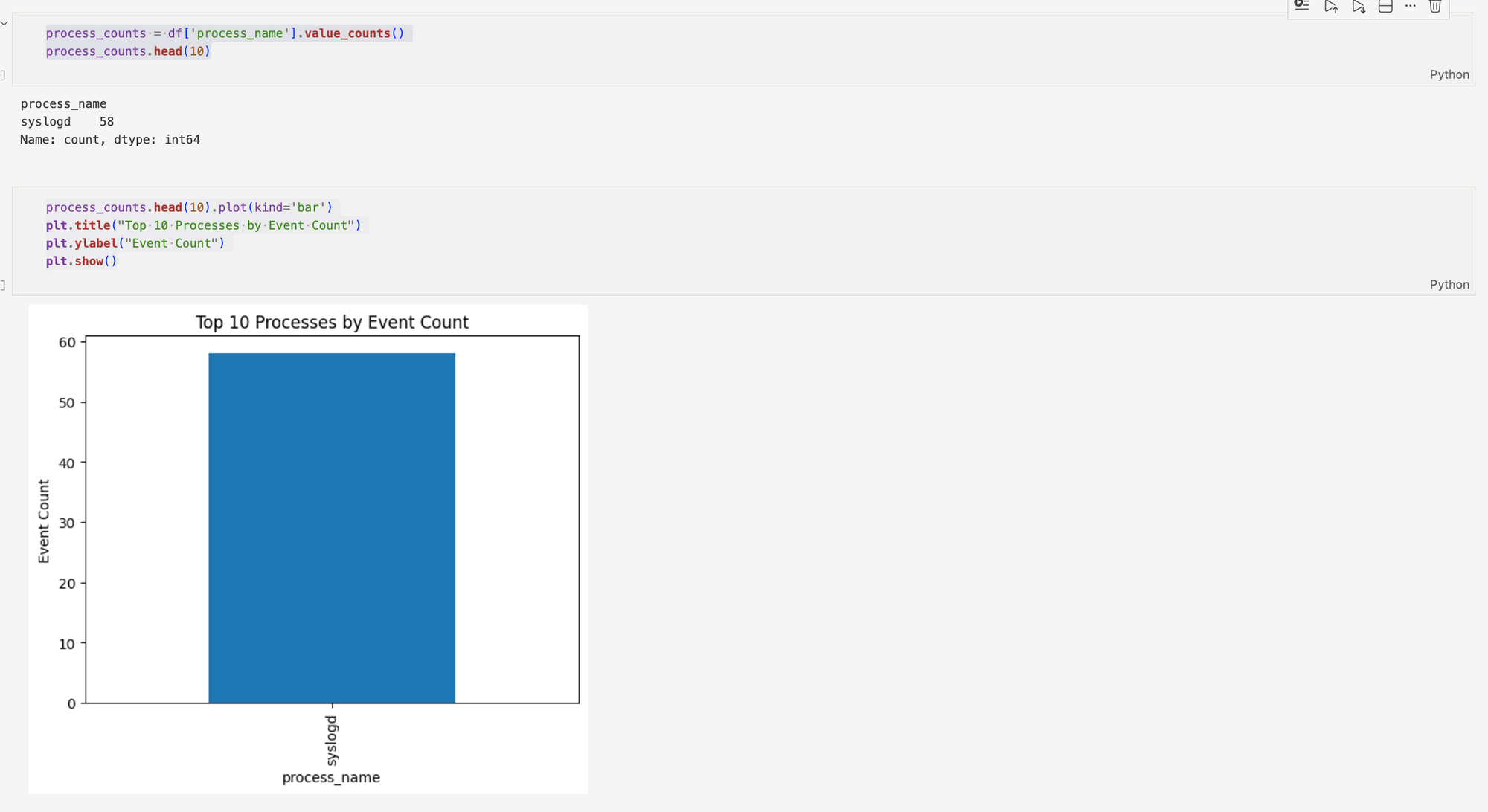
Process frequency is a vital bit of information in order to understand our data. However, all events originate from syslogd, limiting behavioural diversity and reducing the ability to distinguish between different process types. While the data is limited with all processes being syslogd. This highlights a key limitation. A lack of behavioural diversity.
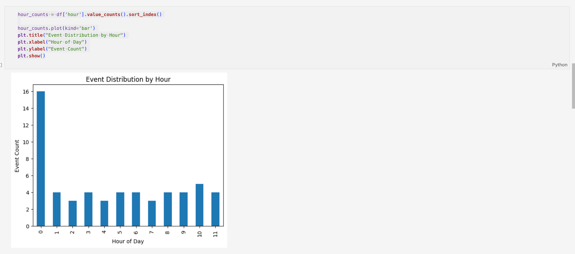
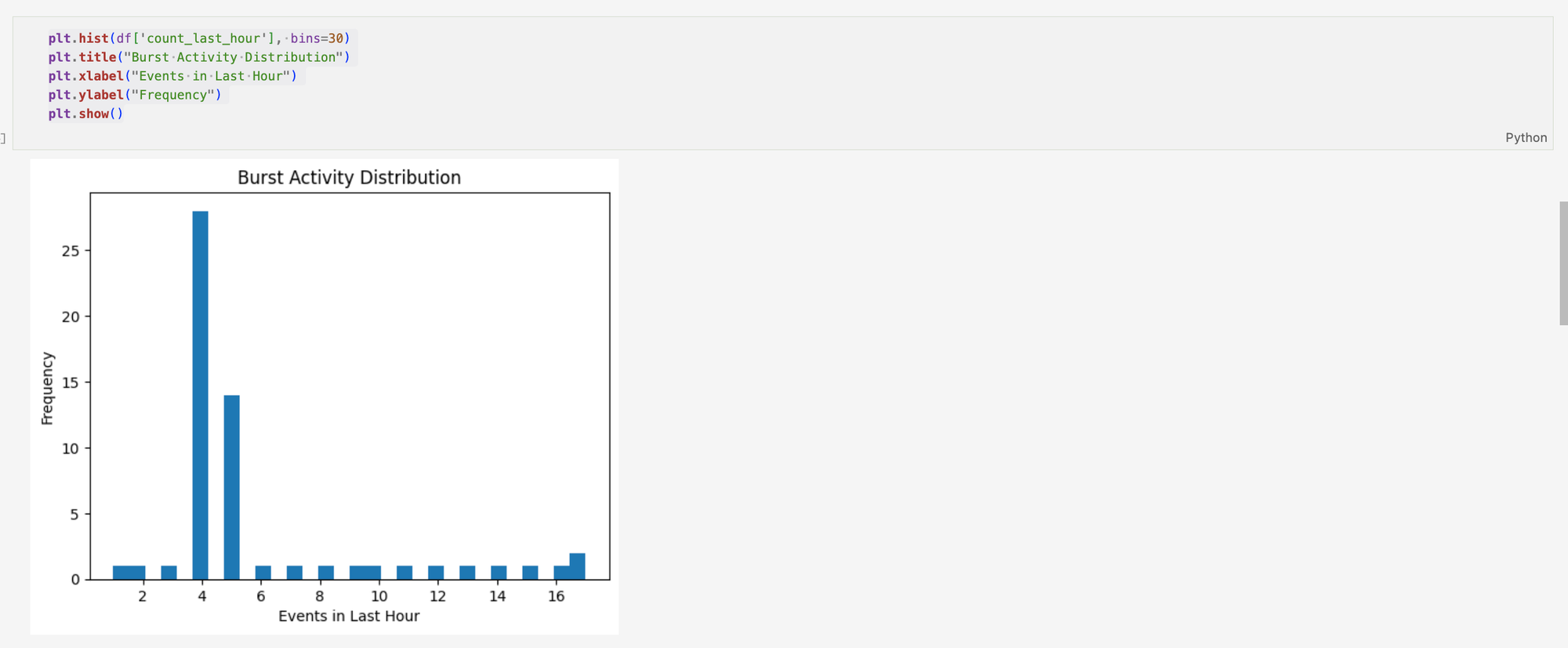
From here, extending my visualisations is very important, this allows for a greater understanding of the data. Event distribution by hour shows where the activity is most concentrated, which shows where system activity is at it's highest. Burst activity shows that there is strong clustering around approximately 4 events in the last hour, which can be interpreted as a relatively stable baseline of activity.
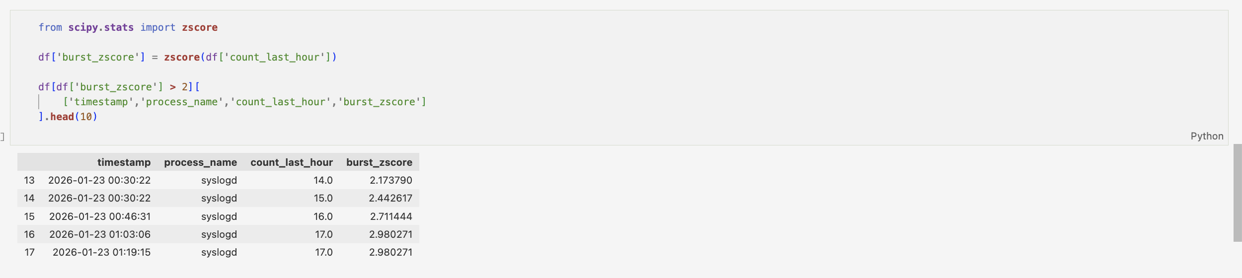
To quantify burst behaviour, a z-score was assigned to count_last_hour feature, allowing values to be standardised relative to overall distribution. Filtering for values greater than 2 allows for analysis of potential burst events, which doesn't definitely indicate anomalous behaviour.

Creating a binary classification system for suspicious action (off_hours, rare_process & burst_zscore). This allows for a more holistic view of system behaviour.
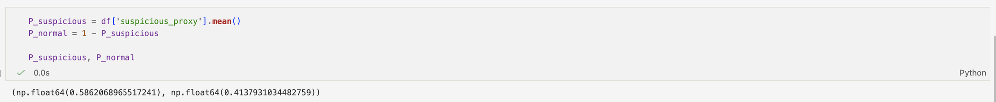
The mean of this binary variable provides an estimate of how frequently the system exhibits at least one unusual characteristic, offering a simple baseline measure of potential anomalous activity.
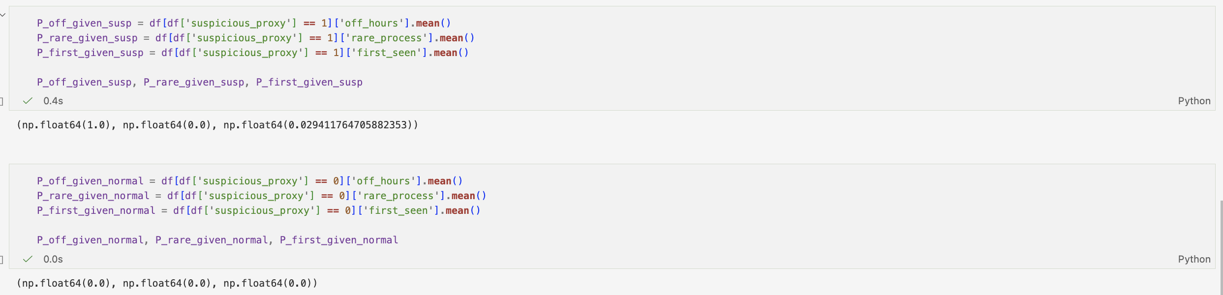
To further our understanding of the data, it was split into two groups, normal and suspicious. Then, using probability measured how often certain behaviours appear in each group — for example, how likely events are to happen at night and involve rare processes.
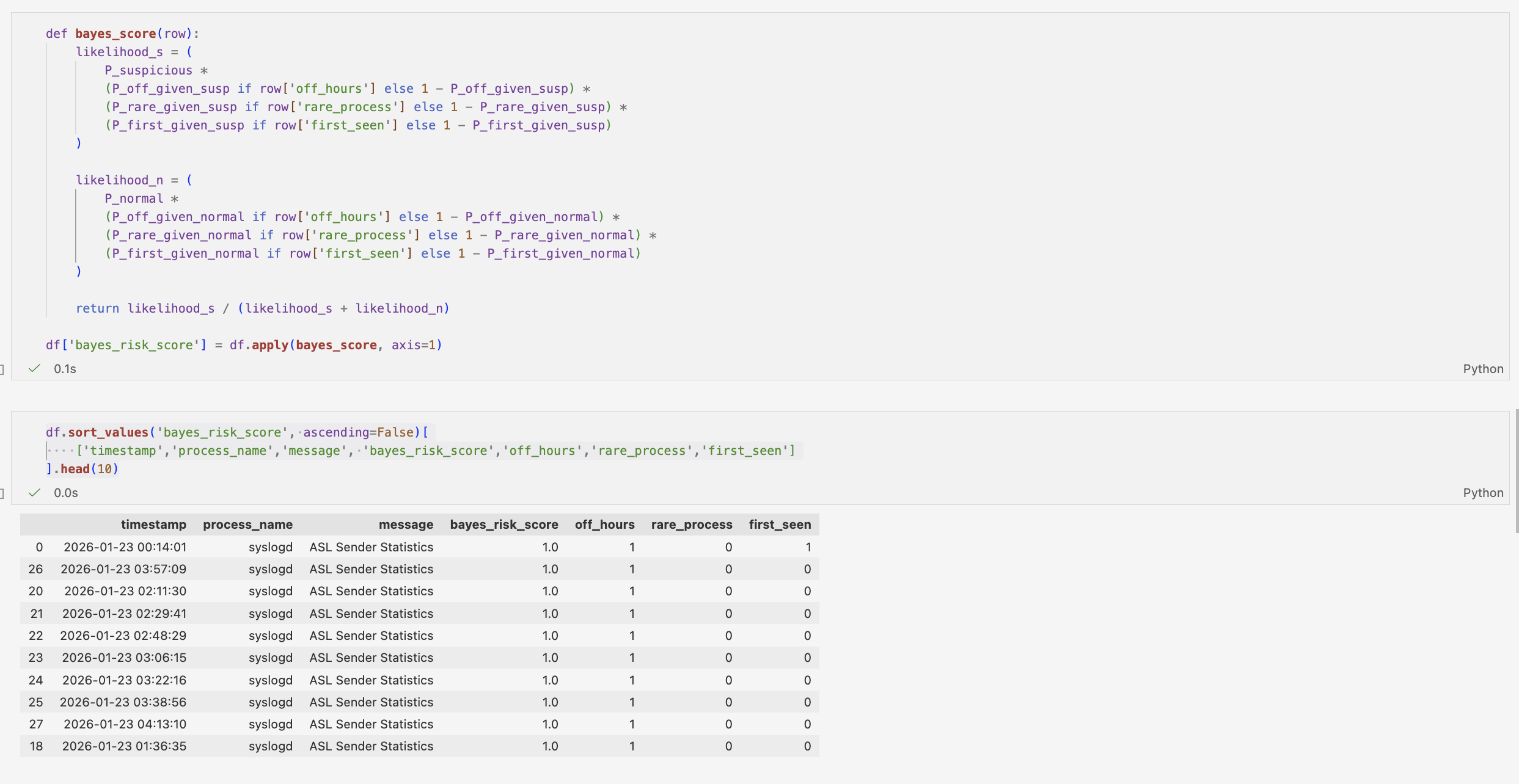
Using a Naive Bayes-inspired approach, each event is assigned a probabilistic risk score. This risk score represents the likelihood of each event being classified as suspicious given its observed features. Then sorting the values based on the top 10, I am able to demonstrate how probabilistic modelling can be used not only to classify events, but to prioritise and rank them by relative risk.
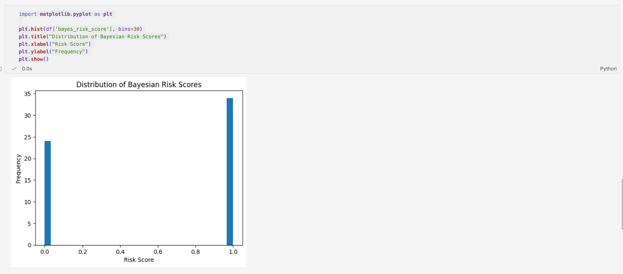
Looking at the distribution of the Bayesian Risk Scores, it shows a binary distribution. This indicates that the model is working effectively, separating the dataset into two dominant behavioural groups: normal and suspicious activity. Rather than producing a continuous range of risk scores, the model assigns each event to one of two clear categories.
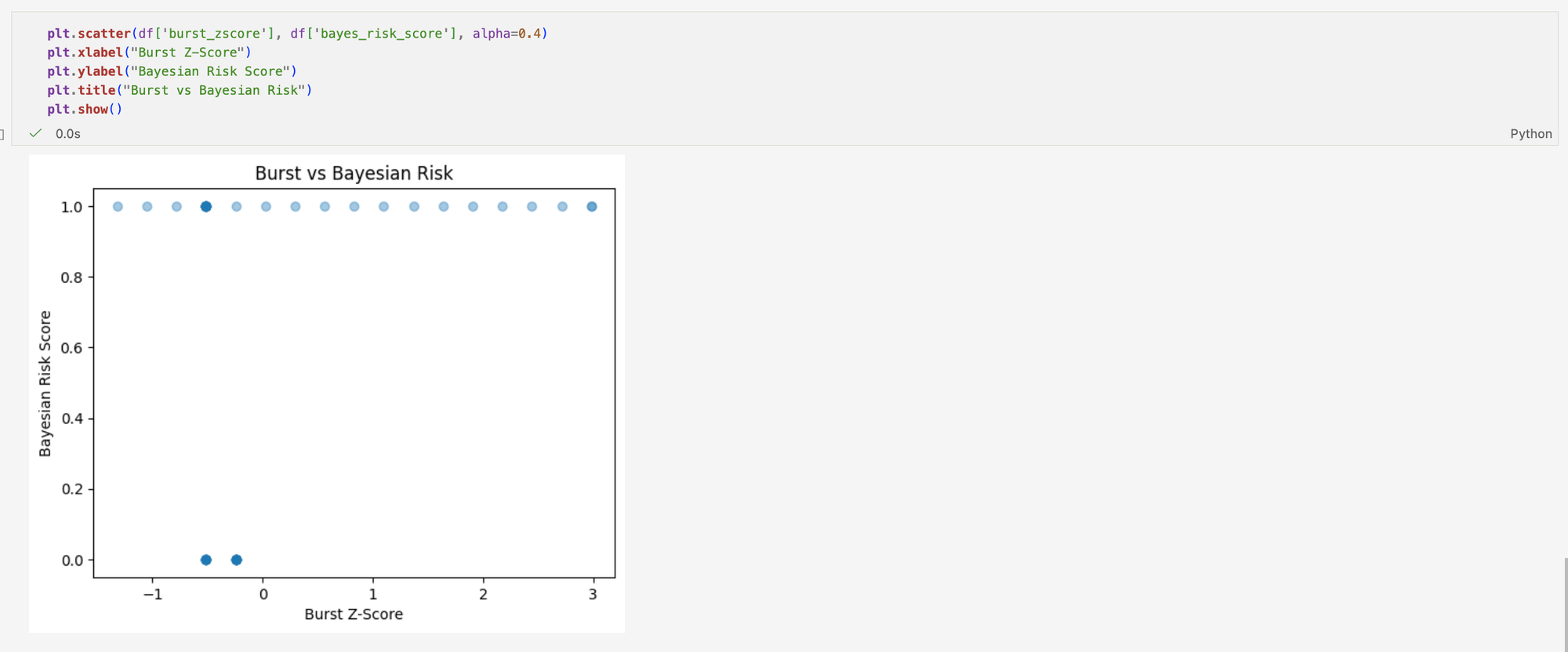
This scatter plot compares statistical anomaly detection (burst z-score) with a rule-based Bayesian risk score across system log events. It shows that many events are flagged as suspicious by the rule-based model, but this does not necessarily indicate true abnormal behaviour in the system; instead, it reflects how frequently predefined conditions are triggered in routine logs.
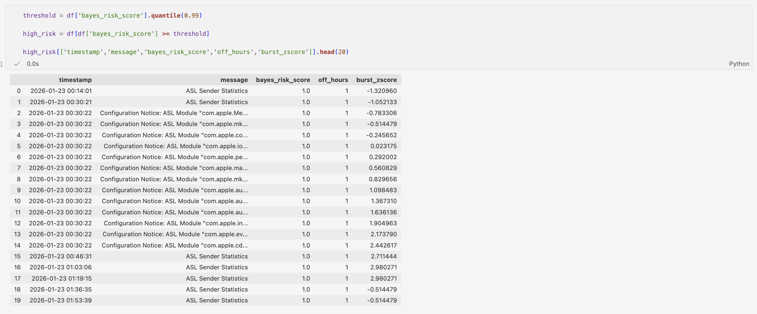
This table shows the top 1% of Bayesian risk events, revealing that while all are flagged as suspicious, their underlying statistical behaviour varies significantly, indicating that the model captures rule activation rather than true anomaly intensity.
Bringing all of this together, this analysis shows that statistical anomaly detection (z-score), rule-based heuristics, and a Naive Bayes-inspired scoring model each produce different interpretations of the same system logs. While the z-score captures deviations in activity volume, the Bayesian model reflects the presence of predefined behavioural triggers such as off-hours or rare process activity. In practice, these approaches do not consistently align, as seen in the high-risk subset where both routine system behaviour and statistically unusual events are grouped under the same “suspicious” label. This highlights a key limitation of simple detection systems: they often reduce complex, continuous system behaviour into binary decisions, which can obscure meaningful distinctions in the underlying data.